DAA(Design Analysis & Algorithms) B.tech 6th sem

 

Dijkstra’s algorithm

• 1.     Dijkstra’s algorithm solves the single-source shortest-paths problem on a weighted, directed graph G = (G, v) for the case in which all edge weights are nonnegative.
• 2.     Dijkstra’s algorithm maintains a set S of vertices whose final shortest-path weights from the source s have already been determined.

Initialize Algorithm:-

Relax Algoritham:-

Example of Relax algorithm

Relaxing an edge (u, v) with weight w(u, v)=2.  The shortest-path estimate of each vertex appears within the vertex.

a a)     Because v.d > u.d + w(u, v) prior to relaxation, the value of v.d decreases.

b)    b) Here v.d <=u.d + w(u, v) before relaxing the edge, and so the relaxation step       leaves v.d unchanged.

Example Of Dijkstra:-

Step1   Initialization:-

Step 2.  set S= { }

Step 3.  

length of(Q)=5

Step 4.  while Q!= nil

              condition true( because 5!=nil)

Step 5.     u=min(Q)       

                 (i.e u= min(s,t,x,y,z)  Firstly s is source vertex so minimum value of s =0)

Step 6.  S=S U {u}

               S=S U {s}

                S=S  (because s union s is equal to s)

Step 7.    vertex v belongs to adj[u] 

                now see the Adjcent vertex of s in above graph i.e t, y

Step 8.    RElAX(u,v,w)    

                update min weight of adjcent vertex in graph

Step 9. Repeat Step 5 to step 8 continuously untill will goes  min weight of all vertex in graph.

 Now min weight of vertex y. so check the adjcent vertex of y in graph i.e  t, x

 so update min weight of adjcent vertex of y in graph.

Step 10.   Now min weight of vertex z. so check the adjcent vertex of t in graph i.e  s, x

 so update min weight of adjcent vertex of z in graph.

Step 11.   Now min weight of vertex t. so check the adjcent vertex of t in graph i.e  y, x

 so update min weight of adjcent vertex of t in graph.

Step 12.   last and  remaining vertex x doest visit. so check the adjcent vertex of x in graph i.e  z  so update min weight of adjcent vertex of z in graph if possible otherwise left.

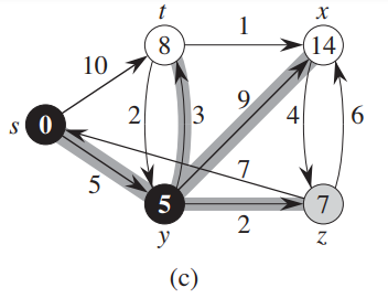
Step13.     Finally Queue is with weighted vertex 

Bellman-Ford algorithm

1.   The Bellman-Ford algorithm solves the single-source shortest-paths problem in the general case in which edge weights may be negative.
2.     If there is such a cycle, the algorithm indicates that no solution exists.
3.    If there is no such cycle, the algorithm produces the shortest paths and their weights.
4. The Bellman-Ford algorithm runs in time O(VE)

Bellman-Ford algorithm

Step1   Initialization:-

Step 2.    RElAX(u,v,w)    

                update min weight  from Source vertex s to vertex t , y  in graph

Step 3.    RElAX(u,v,w)    

                update min weight  from t,y vertex  to vertex x , z in graph

Step 4.    RElAX(u,v,w)    

                update min weight  from x vertex to vertex t in graph

Step 4.    RElAX(u,v,w)    

                update min weight  from t vertex to vertex z in graph

The Bellman-Ford algorithm return ture in this example.

Huffman code

(i) Data can be encoded efficiently using Huffman Codes.

(ii) It is a widely used and beneficial technique for compressing data.

(iii) Huffman's greedy algorithm uses a table of the frequencies of occurrences of each character to build up an optimal way of representing each character as a binary string.

Represent the data in a Compact way:-

(i)               Fixed length Code

(ii)             A variable-length code

Fixed length Code: 

Each letter represented by an equal number of bits. With a fixed length code, at least 3 bits per character:

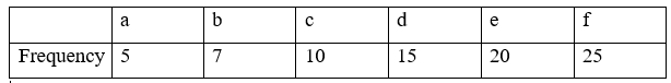
Total frequency = 5 + 7 + 10 + 15 + 20 + 25

                        = 82

Memory required for sending the file = 5*3 + 7*3 + 10*3 + 15*3 + 20*3 + 25*3  (represented by  3bit per character)

                                                            = 246

  A variable-length code: 

It can do considerably better than a fixed-length code, by giving many characters short code words and infrequent character long codewords. It is represented by Huffman tree.

Huffman tree

Case 1: Take minimum 2 frequency character from the above table and merge both of them. Minimum frequency goes to LHS of the tree and maximum frequency goes to RHS of the tree.  continue the..............

·        *   Left edge assign 0 bit and right edge assign 1 bit to all Huffman tree.

     Binary code of Huffman tree characters:-

A : 1010

B : 1011

C : 100

D : 00

E : 01

F : 11

Memory required for sending the file = 5*4 + 7*4 + 10*3 + 15*2 + 20*2 + 25*2 

= 198 bit

Activity Selection problem: -

A set of n jobs/tasks/lecture/games with their starting time (S_i) and finishing time (F_i) is given to us. We want to schedule max. no. without any conflict on single professor / lecture hall / playground.

·        Take first earliest starting time.

·        Minimum conflict

·        Give the optimal solution

Question:-

 

Schedule maximum task using activity problem solution.

Answer:-

1.   First schedule the  task t2 because  earliest starting time( i.e 1) . whenever task         T2 is schedule then T1, T3 and T4 is not schedule because  task T2 finishing         time is 6.  Next task schedule after task t2 finishing time.

2. Second schedule task is  T5

3. Third schedule task is T6

So Maximum schedule task  is 3   i.e  (t2, t5, t6) 

Unit-4

Longest common subsequence(LCS)

1. Subsequence is obtained by dropping few elements from a sequence.

2. Running time or cost is O(n²)

3. LCS[i, j] = the length of LCS of two sequences

Sequence: A       B       A       C      B       D

Subsequence:     B       C       D

Example:

X:      A       B       B       A       C

Y:      B       A       B       C      

LCS(X,Y)    = A, B, C

                    =B, B, C

                    =B, A, C

Applications of Greedy Algorithm

• It is used in finding the shortest path.
• It is used to find the minimum spanning tree using the prim's algorithm or the Kruskal's algorithm.
• It is used in a job sequencing with a deadline.
• This algorithm is also used to solve the fractional knapsack problem.

Unit-5

Branch and Bound 

Branch and bound algorithms are used to find the optimal solution for combinatory, discrete, and general mathematical optimization problems.

Branch and bound is one of the techniques used for problem solving. It is similar to the backtracking since it also uses the state space tree. It is used for solving the optimization problems and minimization problems. If we have given a maximization problem then we can convert it using the Branch and bound technique by simply converting the problem into a maximization problem.

Let's understand through an example.

Jobs = {j1, j2, j3, j4}

P = {10, 5, 8, 3}

d = {1, 2, 1, 2}

The above are jobs, problems and problems given. We can write the solutions in two ways which are given below:

Suppose we want to perform the jobs j1 and j4 then the solution can be represented in two ways:

The first way of representing the solutions is the subsets of jobs.

S1 = {j1, j4}

The second way of representing the solution is that first job is done, second and third jobs are not done, and fourth job is done.

S2 = {1, 0, 0, 1}

The solution s1 is the variable-size solution while the solution s2 is the fixed-size solution.

First, we will see the subset method where we will see the variable size.

First method:

In this case, we first consider the first job, then second job, then third job and finally we consider the last job.

As we can observe in the above figure that the breadth first search is performed but not the depth first search

Different search techniques in branch and bound:

1.     LC search

2.     BFS

3.     DFS

1. LC search (Least Cost Search):

·        It uses a heuristic cost function to compute the bound values at each node.

·         Nodes are added to the list of live nodes as soon as they get generated.

·        The node with the least value of a cost function selected as a next E-node.

2.BFS(Breadth First Search):

·        It is also known as a FIFO search.

·        It maintains the list of live nodes in first-in-first-out order i.e, in a queue, The live nodes are searched in the FIFO order to make them next E-nodes.

 

3. DFS (Depth First Search):

·        It is also known as a LIFO search.

·        It maintains the list of live nodes in last-in-first-out order i.e. in a stack.

·        The live nodes are searched in the LIFO order to make them next E-nodes.